Demystifying Machine Learning: How I Taught a Computer to Predict Pizza Prices
Introduction: Beyond the Black Box
We use Machine Learning every day, but it often feels like magic. To truly understand the "why" behind the magic, I decided to step away from high-level libraries like Scikit-Learn. Instead, I built a Single Variable Linear Regression model from the ground up to solve a vital human dilemma: predicting the price of a pizza based on its diameter.
1. The Model: The Equation of a Line
At its core, simple linear regression is just the equation of a line from high school algebra:
$$f_{w,b}(x) = wx + b$$
- $x$: The input (Pizza diameter).
- $w$: The weight (How much the price increases per inch).
- $b$: The bias (The base cost of the pizza).
- $f_{w,b}(x)$: The prediction (The price).
2. The Scoreboard: The Cost Function
How does the computer know if it’s doing a good job? We use a Cost Function, specifically the Squared Error Cost Function. Think of this as a scoreboard where a high score is bad. The goal of our model is to minimize this "error" score.
Why $1/2m$?
You might notice we divide by $2m$. The $m$ represents the number of training examples, and the $2$ is a mathematical "gift" to ourselves—it cancels out the exponent when we take the derivative during calculus, making our updates much cleaner!
3. The Engine: Gradient Descent
To find the lowest point on our "error scoreboard," we use an optimization algorithm called Gradient Descent.
Imagine you are a hiker in a thick fog on a mountain. You can't see the valley, but you can feel the slope of the ground under your feet. You take a small step in the direction where the slope is steepest downward. You repeat this until you reach the bottom.
In code, the update looks like this:
Python
# Updating the weight
w = w - alpha * dj_dw
# Updating the bias
b = b - alpha * dj_db
Here, alpha ($\alpha$) is our Learning Rate—the size of the step the hiker takes.
4. Visualizing the Results
The most rewarding part of this project was seeing the data come to life.
The Learning Curve
By tracking the cost at every iteration, we can see the model "learning" in real-time. As the iterations increase, the cost drops sharply and then levels off as it finds the optimal parameters.
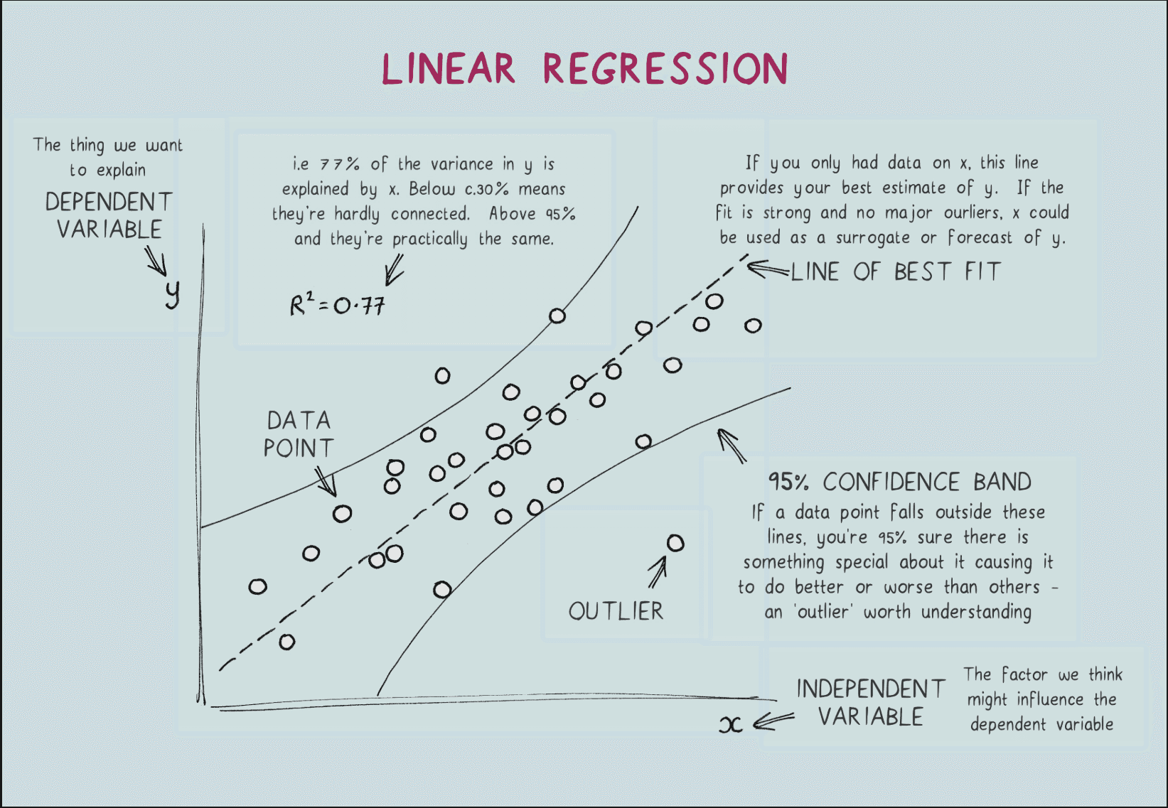
The Line of Best Fit
After 10,000 iterations, the model found the best possible line to represent our pizza data. When I asked it to predict the price of a 15-inch pizza, it gave me a price of $17.88.
Conclusion
Building this from scratch taught me that ML isn't magic—it's iterative optimization and calculus. By adjusting the Learning Rate and watching the gradients, I gained a deep intuition that using a library alone could never provide.